Bike Power and Hills

I’m a cyclist, and I’m also a nerd who loves playing with data, so unsurprisingly, I buy pretty much every kind of sensor I can afford to put on my bike and track various datastreams during my rides. Last year, I finally shelled out for a power meter, generally considered the gold standard type of training data since, unlike speed, power output should be comparable across all kinds of conditions (indoor/outdoor riding, wind speeds, etc.). Through that, I’ve been learning about different ways to use and target different power ranges in training. The standard parlance revolves around “functional threshold power,” or FTP, defined as the steady power output one could theoretically maintain for an hour. Then various effort levels for interval training are done at various multiples of FTP. For indoor training, I’ve actually been using Sufferfest, which does a fitness test designed to find your maximal power over several different durations, based on data suggesting that the maximum power someone can maintain for, say, five minutes, as a multiple of FTP, can vary greatly across individuals. See more here, it’s pretty interesting stuff. Here are my most recent results:

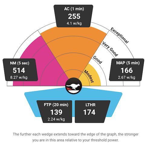
Since I moved to Pittsburgh and have been cycling on some of the abundant hills in this area (I actually had to get some easier gears on my bike for this purpose), it’s been interesting to track all this data as I (oh so very gradually) get better at climbing! On my ride yesterday, I started getting curious about some of the inherent differences between riders with different FTP riding on the same terrain, and also the nonlinearities between power and speed, on those gradients or on a flat road. So I decided to do some physics to it!

The model

NOTE: Thanks a million to Chris White from Ride Far for this PDF that informed my notation here, and more importantly, provided some characteristic values for several of the coefficients about which I had no idea.

All the calculations I allude to below have been done in Python and the code is available on GitHub here, but I’ll include some of it inline in this post too. To start…

from scipy.constants import g, R, atm
import numpy as np
from itertools import product
import pandas as pd
import seaborn as sns
from matplotlib import pyplot as plt

Okay, so let’s lay out these equations. The basic premise of all of this (thanks, Newton) is that if you’re going at a steady speed, the power you are exerting should be equal to the power being dissipated by all the various resistive forces:

So the crux of this is modeling either side of this. Let’s start with the more complicated one, the right side. For this, we need to enumerate every resistive force. First, air resistance:

where $C_dA$ is the product of the drag coefficient and the area (characteristic values for this are tabulated here), $v_a$ is the air speed, and $\rho$ is the air density, which we can model as:

where $p_0$ is a standard atmosphere (101,325 Pa), $R_s$ is the specific gas constant (287.058 J/[kg K]), $L$ is the approximate rate of decrease in temperature with elevation (0.0065 K/m), $h$ is the altitude in meters (about 500 for Pittsburgh), $M$ is the molar mass of dry air (0.02896 kg/mol), and $R_U$ is the universal gas constant (8.315 J/[mol K]).

Here’s the Python code for air resistance:

# air density in kg/m^3
def air_density(altitude=500, T=293):
    L = 0.0065
    T0 = 298
    M = 0.02896
    Rs = 287.058
    p_exp = M*g/(R*L)
    p = atm*(1-(L*altitude/T0))**p_exp
    return p/(Rs*T)

# resisting force from air
def F_air(mph, CdA, rho=air_density()):
    speed = mph/2.237
    return 0.5 * CdA * rho * speed**2

Next, rolling resistance! To compute the rolling friction, we need to know the force normal to the road, hence the triggy stuff.

def F_roll(grad, m, Crr):
    return Crr * np.cos(np.arctan(grad)) * m * g

Here, $C_{rr}$ is the coefficient of rolling resistance (which I could look up for my tires here, it’s 0.00483), and $G$ is the gradient of the road, that is, the tangent of its angle of inclination.

And finally, gravity, for which we need the component along the level of the road:

def F_grav(grad, m):
    return np.sin(np.arctan(grad)) * m * g

We can sum these up and multiply by the ground speed to get the total resistive power:

I’ll also assume for simplicity that $v_g=v_a\equiv v$, i.e. the ground speed is equivalent to the air speed (no wind). Then, the above equation becomes a cubic in the velocity:

We’re almost there! We just need the other side of that original equation, the $P_{wheel}$ part. Unfortunately, all the power I can drive from my legs into my pedal-based power meter does not get to the wheel to drive the bike forward, because drivetrains are not 100% efficient. So we need to account for drivetrain losses $L_{dt}$:

Thanks to Chris White, I now know that a characteristic value for $L_{dt}$ is 0.051, so that’s what I’ve used here.

The results

First, I made a plot of power needed to achieve a given speed on various gradients (for reference, 0.0 is a flat road, 0.06 is usually the highest allowed on US highways, and the steepest hill in Pittsburgh (also the steepest public road in the US) is Canton Avenue which purportedly reaches a grade of 0.37):

def P_needed(mph, grad, m, CdA, Crr, rho, L_dt=0.051):
    speed = mph/2.237 # convert to m/s
    F_resist = F_air(mph, CdA, rho) + F_roll(grad, m, Crr) + F_grav(grad, m)
    return F_resist * speed / (1.0-L_dt)

mph_vals = np.arange(4,12.1,0.1)
grad_vals = np.arange(0.0, 0.25, 0.03)
df = pd.DataFrame.from_records(data=[p for p in product(mph_vals, grad_vals)], columns=["speed", "gradient"])
# calculate for me and my bike
df['W/kg'] = [Wperkg(63.5, 8.0, a.speed, a.gradient) for a in df.itertuples()]
sns.lineplot(x='speed', y='W/kg', data=df, hue='gradient', palette=sns.cubehelix_palette(len(grad_vals), start=0, rot=.5))
# plus some plot formatting stuff

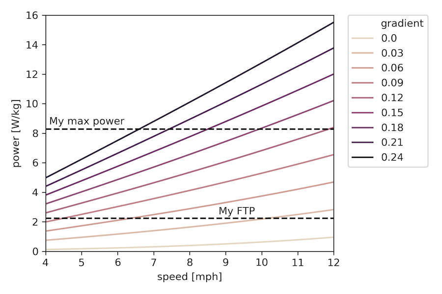
Note that the y-axis here is in watts per kilogram of body mass, so things will shift a bit if the ratio of body mass to bike (+gear) mass changes, for the calculations here it was about a factor of 9. I also put my FTP and my maximum 5-second power on as reference points. The choice of x-axis lower limit was also deliberate, as in my experience, 4 mph is about the slowest one can go uphill and remain upright.

So this plot certainly shows some of the things I’d been thinking about – for example, if we consider FTP to be some measure of “sustainable” power output, then we can get a sense of what grades folks with different FTP values can sustainbly chug their way up for quite awhile while staying above that 4mph threshold. For me at 2.24, it’s something like 9-10% or so. Whereas if you’re a much fitter person than I, you might be able to go up that 9% in excess of 10 mph at your FTP, or alternatively, at around the same pace on something like a 15% grade.

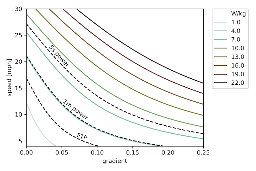
This is cool, but I realized I actually wanted a different chart, one where we could explicitly see the tradeoff between speed and gradient for a fixed power. To do that, we need to solve the cubic equation I outlined above. Fortunately, it always has exactly one real root, so that’s pretty easy, and we can make this plot (we’re essentially showing where different horizontal lines on the previous plot intersect with the curves for different gradients):

def calc_speed(watts_per_kg, grad, body_mass, bike_mass, CdA=0.45, Crr=0.00483, rho=air_density(), L_dt=0.051):
    total_mass = body_mass + bike_mass
    a3 = 0.5*CdA*rho
    a1 = F_roll(grad, total_mass, Crr) + F_grav(grad, total_mass)
    a0 = -1.0 * watts_per_kg*body_mass * (1.0-L_dt)
    rts = np.roots([a3, 0, a1, a0])
    # one should be real, return that one
    return [r.real*2.237 for r in rts if r.imag==0][0]

    P_vals = np.arange(1.0,22.1,3.0)
    grad_vals = np.arange(0.0,0.252,0.002)
    df = pd.DataFrame.from_records(data=[p for p in product(P_vals, grad_vals)], columns=["W/kg", "gradient"])
    df['mph'] = [calc_speed(a[1], a.gradient, 63.5, 8.0) for a in df.itertuples()]

sns.lineplot(x='gradient', y='mph', data=df, hue='W/kg', palette=sns.cubehelix_palette(len(P_vals), start=0.2, rot=1.0))
# plus some more beautification

(Sidenote: Cubehelix color palettes are so cool! As is Seaborn generally for dataviz.)

Here now I’ve overlaid my own FTP, maximum 1-minute, and maximum 5-second power values as additional iso-lines. Again, the minimum speed shown is 4mph. For some typical numbers for male and female cyclists of various calibers, check out the chart partway down this page.

In this plot, it’s even easier to read off the kind of things I was discussing above, and also to draw conclusions about what kind of gradients one could “power up” for really short periods of time. For example, if your absolute maximum power output were 4 W/kg, you’re not going to be able to get up anything steeper than around 19%, even instantaneously.

All this analysis is cool, and also serves as a good motivator to get out and improve my power numbers! Especially since the iso-power slopes at the bottom of this curve are such that a relatively small improvement in power capability leads to a comparatively large one in accessible gradients, and I’d love to take a shot at the Dirty Dozen someday!

Reminder that the code is all here so you should definitely go play and put in your own numbers to see how this turns out for you!

Caveats!

In any simple model like this, there are a lot of assumptions! Here is a not-necessarily-exhaustive list

• I ignored the effects of wind (as mentioned above, assumed ground speed equal to air speed)
• I assumed perfectly smooth power profiles, which really only happens if you have ideal pedaling technique – in reality, most of us fluctuate through the pedal stroke, though it’s debatable to what extent one’s power meter can accurately pick this up, and so the average numbers on both ends probably work out decently
• I used $C_dA=0.45$ everywhere since I usually ride in my tops up difficult hills (see graph here), but in reality, on less steep hills, I might be in the hoods or even down in my aerobars, so the speed curves would shift up a little from the reduced air resistance there